

language: en
tags:
  - Clsssification
license: apache-2.0
datasets:
  - tensorflow
  - numpy
  - keras
  - pandas
  - openpyxl
  - gensin
  - contractions
  - nltk
  - spacy
thumbnail: https://github.com/Marcosdib/S2Query/Classification_Architecture_model.png

MCTI Text Classification Task (uncased)
Disclaimer: The Brazilian Ministry of Science, Technology, and Innovation (MCTI) has partially supported this project.
The model NLP MCTI Classification Multi is part of the project Research Financing Product Portfolio (FPP) focuses on the task of Text Classification and explores different machine learning strategies to classify a small amount of long, unstructured, and uneven data to find a proper method with good performance. Pre-training and word embedding solutions were used to learn word relationships from other datasets with considerable similarity and larger scale. Then, using the acquired resources, based on the dataset available in the MCTI, transfer learning plus deep learning models were applied to improve the understanding of each sentence.
According to the abstract,
Compared to the 81% baseline accuracy rate based on available datasets and the 85% accuracy rate achieved using a Transformer-based approach, the Word2Vec-based approach improved the accuracy rate to 93%, according to "Using transfer learning to classify long unstructured texts with small amounts of labeled data".
Model description
After the embedding, which is just essentially data preprocessing, it is necessary to develop the Project further to analyze the input text and classify whether it is a valid research funding opportunity for Brazilian or not.
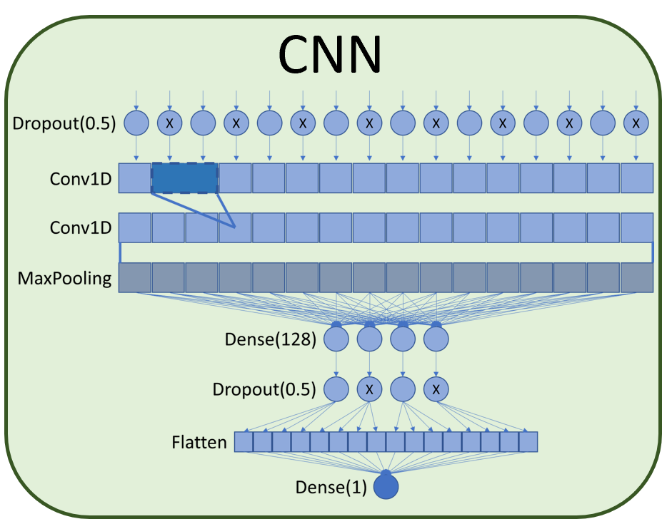
For the project, the best option would be chosen empirically upon comparing the results of 4 distinct architectures: Neural Network (NN), Deep Neural Network (DNN), Long Short-Term Memory (LSTM), and Convolutional Neural Network (CNN). Figure 4 shows the structure of the models.
A neural network (NN) here is a simple feedforward neural network with only a single hidden layer, usually called ”shallow”. Shallow NNs are often limited in the complexity of the problems they can be trained to solve well.
Our CNN model uses a dropout layer feeding into a couple of Conv1D layers and then a MaxPooling layer. After that, we Figure 4: Classification models use a hidden layer composed of a dense layer of size 128, followed by another dropout layer, and finally, the Flatten and final dense classification layer.
The architecture of the CNN network used is composed of a 50% dropout layer followed by two 1D convolution layers associated with a MaxPooling layer. After max pooling a dense layer of size 128 was added connected to a 50% dropout which finally connects to a flatten layer and the final classification dense layer. Dropout layers help to avoid overfitting the network by masking part of the data so that the network learns to create redundancies in the analysis of the inputs.
Model variations
With the motivation to increase accuracy obtained with baseline implementation, was implemented a transfer learning strategy under the assumption that small data available for training was insufficient for adequate embedding training. In this context, was considered two approaches:
- Pre-training word embeddings using similar datasets for text classification;
- Using transformers and attention mechanisms (Longformer) to create contextualized embeddings.
Templates using Word2Vec and Longformer also need to be loaded and their weights are as follows:
Table 1: Templates using Word2Vec and Longformer
| Tamplates | weights |
|---|---|
| Longformer | 10.9GB |
| Word2Vec | 56.1MB |
Intended uses
How to use
You can use this model directly with a pipeline for masked language modeling:
Here is how to use this model to get the features of a given text in PyTorch:
and in TensorFlow:
Limitations and bias
This model is uncased: it does not make a difference between english and English.
Even if the training data used for this model could be characterized as fairly neutral, this model can have biased predictions:
Performance limiting: Loading the longformer model in memory means needing 11Gb available only for the model, without considering the weight of the deep learning network. For training this means we need a 20+ Gb GPU to perform the training. Here this was resolved using the high RAM environment of google Colab Pro and training using CPU which justifies the longer training time per season.
Replicability limitation: Due to the simplicity of the keras embedding model, we are using one hot encoding, and it has a delicate problem for replication in production. This detail is pending further study to define whether it is possible to use one of these models.
- This bias will also affect all fine-tuned versions of this model.
Training data
The inputted training data was obtained from scrapping techniques, over 30 different platforms e.g. The Royal Society, Annenberg foundation, and contained 928 labeled entries (928 rows x 21 columns). Of the data gathered, was used only the main text content (column u). Text content averages 800 tokens in length, but with high variance, up to 5,000 tokens.
Training procedure
Model training with Word2Vec embeddings
After the pre-trained model of word2vec embeddings had already learned meanings relevant to the classification problem, it was coupled to the classification model to train it with the labeled data in a supervised way. Table 6 shows the results obtained with related metrics. With this implementation, was reached new levels of accuracy with 86% for CNN architecture and 88% for the LSTM architecture.
Preprocessing
Pre-processing was used to standardize the texts for the English language, reduce the number of insignificant tokens and optimize the training of the models.
The following assumptions were considered:
- The Data Entry base is obtained from the result of Goal 4.
- Labeling (Goal 4) is considered true for accuracy measurement purposes;
- Preprocessing experiments compare accuracy in a shallow neural network (SNN);
- Pre-processing was investigated for the classification goal.
From the Database obtained in Goal 4, stored in the project's GitHub, a Notebook was developed in Google Colab to implement the preprocessing code, which also can be found on the project's GitHub.
Several Python packages were used to develop the preprocessing code:
Table 2: Python packages used
| Objective | Package |
|---|---|
| Resolve contractions and slang usage in text | contractions |
| Natural Language Processing | nltk |
| Others data manipulations and calculations included in Python 3.10: io, json, math, re (regular expressions), shutil, time, unicodedata; | numpy |
| Data manipulation and analysis | pandas |
| http library | requests |
| Training model | scikit-learn |
| Machine learning | tensorflow |
| Machine learning | keras |
| Translation from multiple languages to English | translators |
As detailed in the notebook on GitHub, in the pre-processing, code was created to build and evaluate 8 (eight) different bases, derived from the base of goal 4, with the application of the methods shown in Figure 2.
Table 3: Preprocessing methods evaluated
| id | Experiments |
|---|---|
| Base | Original Texts |
| xp1 | Expand Contractions |
| xp2 | Expand Contractions + Convert text to lowercase |
| xp3 | Expand Contractions + Remove Punctuation |
| xp4 | Expand Contractions + Remove Punctuation + Convert text to lowercase |
| xp5 | xp4 + Stemming |
| xp6 | xp4 + Lemmatization |
| xp7 | xp4 + Stemming + Stopwords Removal |
| xp8 | ap4 + Lemmatization + Stopwords Removal |
First, the treatment of punctuation and capitalization was evaluated. This phase resulted in the construction and evaluation of the first four bases (xp1, xp2, xp3, xp4).
Then, the content simplification was evaluated, from the xp4 base, considering stemming (xp5), Lemmatization (xp6), stemming + stopwords removal (xp7), and Lemmatization + stopwords removal (xp8).
All eight bases were evaluated to classify the eligibility of the opportunity, through the training of a shallow neural network (SNN – Shallow Neural Network). The metrics for the eight bases were evaluated. The results are shown in Table 4.
Table 4: Results obtained in Preprocessing
| id | Experiment | acurácia | f1-score | recall | precision | Média(s) | N_tokens | max_lenght |
|---|---|---|---|---|---|---|---|---|
| Base | Original Texts | 89,78% | 84,20% | 79,09% | 90,95% | 417,772 | 23788 | 5636 |
| xp1 | Expand Contractions | 88,71% | 81,59% | 71,54% | 97,33% | 414,715 | 23768 | 5636 |
| xp2 | Expand Contractions + Convert text to lowercase | 90,32% | 85,64% | 77,19% | 97,44% | 368,375 | 20322 | 5629 |
| xp3 | Expand Contractions + Remove Punctuation | 91,94% | 87,73% | 79,66% | 98,72% | 386,650 | 22121 | 4950 |
| xp4 | Expand Contractions + Remove Punctuation + Convert text to lowercase | 90,86% | 86,61% | 80,85% | 94,25% | 326,830 | 18616 | 4950 |
| xp5 | xp4 + Stemming | 91,94% | 87,68% | 78,47% | 100,00% | 257,960 | 14319 | 4950 |
| xp6 | xp4 + Lemmatization | 89,78% | 85,06% | 79,66% | 91,87% | 282,645 | 16194 | 4950 |
| xp7 | xp4 + Stemming + Stopwords Removal | 92,47% | 88,46% | 79,66% | 100,00% | 210,320 | 14212 | 2817 |
| xp8 | ap4 + Lemmatization + Stopwords Removal | 92,47% | 88,46% | 79,66% | 100,00% | 225,580 | 16081 | 2726 |
Even so, between these two excellent options, one can judge which one to choose. XP7: It has less training time, less number of unique tokens. XP8: It has smaller maximum sizes. In this case, the criterion used for the choice was the computational cost required to train the vector representation models (word-embedding, sentence-embeddings, document-embedding). The training time is so close that it did not have such a large weight for the analysis.
As a last step, a spreadsheet was generated for the model (xp8) with the fields opo_pre and opo_pre_tkn, containing the preprocessed text in sentence format and tokens, respectively. This database was made available on the project's GitHub with the inclusion of columns opo_pre (text) and opo_pre_tkn (tokenized).
Pretraining
Since labeled data is scarce, word-embeddings was trained in an unsupervised manner using other datasets that contain most of the words it needs to learn. The idea implemented was based on introducing better and better-trained word embeddings in the model. For an additional dataset to be applied to improve word-embedding training, it must be compatible with the dataset used to train the classifier. Was searched for datasets from the Kaggle, a platform with over a thousand available NLP datasets, and the closest we found was the BBC News Articles dataset, which achieved only 56% compatibility.
The alternative was to use web scraping algorithms to acquire more unlabeled data from the same sources, thus ensuring compatibility. The original dataset had 260 labeled entries.
Table 5: Compatibility results (*base = labeled MCTI dataset entries)
| Dataset | |
|---|---|
| Labeled MCTI | 100% |
| Full MCTI | 100% |
| BBC News Articles | 56.77% |
| New unlabeled MCTI | 75.26% |
Table 6: Results from Pre-trained WE + ML models
| ML Model | Accuracy | F1 Score | Precision | Recall |
|---|---|---|---|---|
| NN | 0.8269 | 0.8545 | 0.8392 | 0.8712 |
| DNN | 0.7115 | 0.7794 | 0.7255 | 0.8485 |
| CNN | 0.8654 | 0.9083 | 0.8486 | 0.9773 |
| LSTM | 0.8846 | 0.9139 | 0.9056 | 0.9318 |
Evaluation results
The table below presents the results of accuracy, f1-score, recall and precision obtained in the training of each network. In addition, the necessary times for training each epoch, the data validation execution time and the weight of the deep learning model associated with each implementation were added.
Table 7: Results of experiments
| Model | Accuracy | F1-score | Recall | Precision | Training time epoch(s) | Validation time (s) | Weight(MB) |
|---|---|---|---|---|---|---|---|
| Keras Embedding + SNN | 92.47 | 88.46 | 79.66 | 100.00 | 0.2 | 0.7 | 1.8 |
| Keras Embedding + DNN | 89.78 | 84.41 | 77.81 | 92.57 | 1.0 | 1.4 | 7.6 |
| Keras Embedding + CNN | 93.01 | 89.91 | 85.18 | 95.69 | 0.4 | 1.1 | 3.2 |
| Keras Embedding + LSTM | 93.01 | 88.94 | 83.32 | 95.54 | 1.4 | 2.0 | 1.8 |
| Word2Vec + SNN | 89.25 | 83.82 | 74.15 | 97.10 | 1.4 | 1.2 | 9.6 |
| Word2Vec + DNN | 90.32 | 86.52 | 85.18 | 88.70 | 2.0 | 6.8 | 7.8 |
| Word2Vec + CNN | 92.47 | 88.42 | 80.85 | 98.72 | 1.9 | 3.4 | 4.7 |
| Word2Vec + LSTM | 89.78 | 84.36 | 75.36 | 95.81 | 2.6 | 14.3 | 1.2 |
| Longformer + SNN | 61.29 | 0 | 0 | 0 | 128.0 | 1.5 | 36.8 |
| Longformer + DNN | 91.93 | 87.62 | 80.37 | 97.62 | 81.0 | 8.4 | 12.7 |
| Longformer + CNN | 94.09 | 90.69 | 83.41 | 100.00 | 57.0 | 4.5 | 9.6 |
| Longformer + LSTM | 61.29 | 0 | 0 | 0 | 13.0 | 8.6 | 2.6 |
The results obtained surpassed those achieved in goal 6 and goal 9, with the best accuracy obtained of 94% in the longformer + CNN model. We can also observe that the models that achieved the best results were those that used the CNN network for deep learning.
In addition, it was possible to notice that the model of longformer + SNN and longformer + LSTM were not able to learn. Perhaps the models need some adjustments, but each training attempt took between 5 and 8 hours, which made it impossible to try to adjust when other models were already showing promising results.
Above the results obtained, it is also necessary to highlight two limitations found for the replication and training of networks:
These 10Gb of the model exceed the Github limit and did not go to the repository, so to run the system we need to download the pre-trained network in the notebook and run the encoder-decoder with the data to create the model. It is advisable to do this in a GPU environment and save the file on the drive. After that change the environment to CPU to perform the training. Trying to generate the model in CPU will take more than 3 hours of processing.
The best model that does not have any limitations is Word2Vec + CNN. However, we need to study the limitations to understand whether it is possible to introduce a new model with better accuracy and indicators. These adjustments will be worked on during goals 13 and 14 where the main objective will be to encapsulate the solution in the most suitable way for use in production.
Benchmarks
BibTeX entry and citation info
@conference{webist22,
author       ={Carlos Rocha. and Marcos Dib. and Li Weigang. and Andrea Nunes. and Allan Faria. and Daniel Cajueiro.
               and Maísa {Kely de Melo}. and Victor Celestino.},
title        ={Using Transfer Learning To Classify Long Unstructured Texts with Small Amounts of Labeled Data},
booktitle    ={Proceedings of the 18th International Conference on Web Information Systems and Technologies - WEBIST,},
year         ={2022},
pages        ={201-213},
publisher    ={SciTePress},
organization ={INSTICC},
doi          ={10.5220/0011527700003318},
isbn         ={978-989-758-613-2},
issn         ={2184-3252},
}